Two-Dimensional Lookup
A step-by-step guide to two-dimensional lookups in Excel: combine VLOOKUP with MATCH to retrieve a value by row and column, keep the formula dynamic, and tidy it with nesting.

Xian Hui
23 June 2025
Quick answer
How do you perform a two-dimensional lookup in Excel?
A two-dimensional lookup finds a value by both its row and its column, such as a price for a given product and country. In Excel, the most efficient method combines VLOOKUP with MATCH: VLOOKUP locates the row, while MATCH returns the column position dynamically. This keeps the formula accurate when the lookup criteria change, without adjusting the column number by hand each time.
Two-Dimensional Lookup
Written by Ng Xian Hui, Founder of Backbone. Originally published on ISCA's Chartered Accountants Lab.
In a previous article comparing XLOOKUP and VLOOKUP, I mentioned that XLOOKUP is generally more efficient, except for two-dimensional lookups. But what exactly does that mean, and how do you build one? This article walks through the method, using a small pricing table as the example.
Key takeaways
- VLOOKUP combined with MATCH is the best approach for two-dimensional lookups in Excel.
- MATCH makes VLOOKUP dynamic, removing the need to adjust the column number by hand.
- Nesting the two functions improves clarity, but excessive nesting reduces readability.
- XLOOKUP needs a column reference rather than an index number, which makes it less efficient here.
What is a two-dimensional lookup, and why does the table matter?
Many of the data tables we use in accounting are two-dimensional, which makes them easier to read. Take a pricing table that lists products down the side and countries across the top. Most accountants prefer the layout of Table 1 over the flat list in Table 2.
Table 1
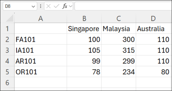
Table 2
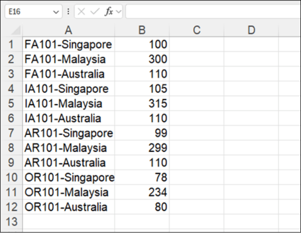
Table 1 is more human-friendly, but it is not ideal for Excel's lookup functions, which are built to read down a single column. If you prefer not to unpivot the table but still want to pull out individual values automatically, read on.
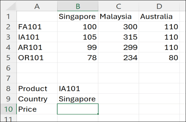
In the example below, the lookup area sits underneath the data: the product goes in cell B8, the country in cell B9, and the price we want to return appears in cell B10.
Table 3
How do you use VLOOKUP for a two-way lookup?
Let's find the price of product IA101 for Singapore.
VLOOKUP helps you find values in a table. It takes four arguments:
- Lookup value — the value to search for.
- Table array — the range of data to search within.
- Column index number — the column from which to return the value.
- Range lookup — use 0 or FALSE for an exact match.
Written out, the function looks like this:
=VLOOKUP(lookup_value, table_array, col_index_num, [range_lookup])For IA101 in Singapore, Singapore is the second column of prices, so the column index number is 2:
=VLOOKUP(B8, A1:D5, 2, FALSE)This returns 105, the correct price.
Table 4
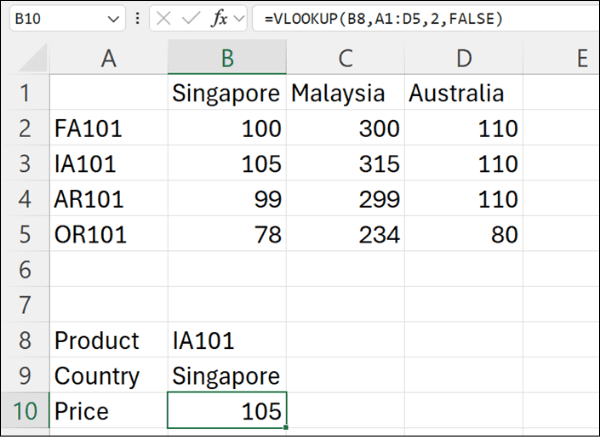
The problem is the fixed number 2. Nobody wants to edit the formula every time the country changes. We need a dynamic column index number for the third argument instead of a static one. But how do we make it dynamic?
How does MATCH make VLOOKUP dynamic?
MATCH is the best companion for VLOOKUP. It works out the relative position of a lookup value within a range. Unlike VLOOKUP, it does not return the value itself but its position — which is exactly what we need to select the right column automatically.
The MATCH function takes three arguments:
=MATCH(lookup_value, lookup_array, match_type)- Lookup value — the value to search for, such as the country name.
- Lookup array — the range containing the column headers, such as a row of country names.
- Match type — use 0 or FALSE for an exact match.
We use MATCH to find the column number for Singapore, so that when the criteria change, the column number updates on its own:
=MATCH(B9, A1:D1, 0)The result is 2, which is correct, since Singapore is the second column in the table.
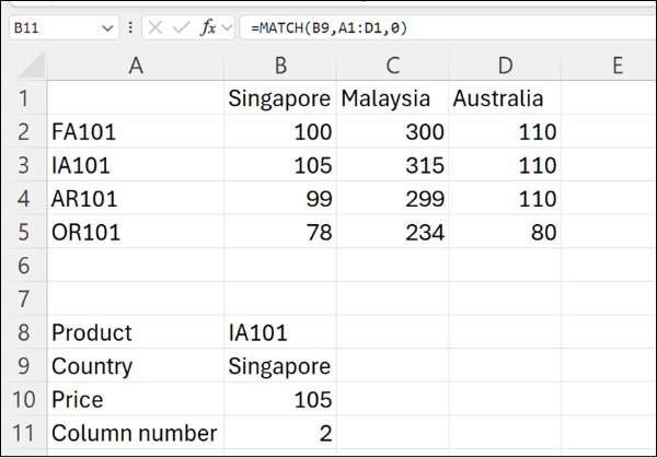
Now return to the VLOOKUP formula and replace the third argument with a reference to the MATCH result in cell B11:
=VLOOKUP(B8, A1:D5, B11, FALSE)Table 6
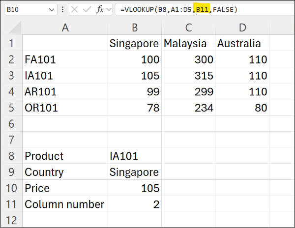
With this setup, changing the country in cell B9 automatically updates the VLOOKUP result. There is no longer any need to adjust column numbers by hand.
How do you nest the formulas for a cleaner worksheet?
Now let's streamline the formula into a single cell. This technique is called nesting.
Nesting one function inside another is straightforward. Experienced users can drop MATCH straight into VLOOKUP but, if nesting is new to you, follow this approach. Since the VLOOKUP formula references cell B11, copy the MATCH formula from B11 (excluding the equals sign) and paste it in place of the reference to B11. You can then delete cell B11 entirely.
=VLOOKUP(B8, A1:D5, MATCH(B9, A1:D1, 0), FALSE)Table 7
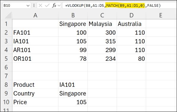
Nesting makes a worksheet look tidier. Nesting two functions is usually fine, but avoid excessive nesting: it can make formulas overly complex, reduce readability, and make future amendments harder.
Why isn't XLOOKUP preferred here?
XLOOKUP is a powerful function, but in this case it does not offer the same efficiency as VLOOKUP. The key difference is how each one specifies the column to return:
- VLOOKUP requires a column index number.
- XLOOKUP requires a column reference.
To work out a relative column index dynamically, we can use MATCH, which is efficient. To work out a dynamic column reference for XLOOKUP, we would need OFFSET — a volatile function — or a second nested INDEX and MATCH.
The table below summarises the trade-off.
| Function pairing | How the column is chosen | Drawback for two-dimensional lookups |
|---|---|---|
| VLOOKUP + MATCH | Column index number from MATCH | None significant; MATCH is lightweight |
| XLOOKUP + OFFSET | Column reference from OFFSET | OFFSET is volatile and recalculates often |
| XLOOKUP + INDEX + MATCH | Column reference from INDEX and MATCH | Extra nesting adds calculations |
Excessive use of volatile functions can cause performance issues and slow recalculation. Extra nested functions increase the number of calculations Excel must perform. For those reasons, VLOOKUP combined with MATCH is the better choice for handling two-dimensional lookups efficiently.
Which approach should you use?
For a two-dimensional lookup — retrieving a value by both its row and its column — reach for VLOOKUP with MATCH. VLOOKUP finds the row, MATCH supplies the column index dynamically, and nesting the two keeps everything in one clean cell. Save XLOOKUP for the many other lookups where its separate lookup and return arrays make it the simpler tool.
References
- Microsoft, VLOOKUP function.
- Microsoft, MATCH function.
Frequently asked questions
This information has been prepared for general informational purposes only and is not intended to be relied upon as accounting, tax, or other professional advice.
Related articles
articles
Advanced Lookup: Wildcards
How accountants use Excel wildcards — the asterisk and question mark — to match account names and codes by pattern in SUMIF, VLOOKUP and XLOOKUP formulas.
articles
Dynamic Array Formulas in Excel: Unleashing the Power
How Excel dynamic array formulas such as FILTER and XLOOKUP spill results across cells, so accountants can build scalable, error-resistant templates and audit working papers.
articles
Multiple Criteria VLOOKUP Guide
How to run a lookup on more than one criterion in Excel — by combining fields into a single identifier, or by using functions built for multiple criteria such as SUMIFS and FILTER.