Multiple Criteria VLOOKUP Guide
How to run a lookup on more than one criterion in Excel — by combining fields into a single identifier, or by using functions built for multiple criteria such as SUMIFS and FILTER.

Xian Hui
23 June 2025
Quick answer
How do you perform a lookup with multiple criteria in Excel?
Most Excel lookup functions, including VLOOKUP, accept only one lookup criterion. To match on several criteria, either combine the fields into a single unique identifier and look up that value, or use functions built for multiple conditions, such as SUMIFS and FILTER. SUMIFS suits numerical data, while FILTER can return whole rows but has more complex syntax.
Multiple Criteria VLOOKUP Guide
Written by Ng Xian Hui, Founder of Backbone. Originally posted on Chartered Accountants Lab (ISCA).
Key takeaways
- In Excel, most lookup functions are designed to accept only a single lookup criterion. But in accounting, scenarios frequently arise where multiple criteria are essential.
- The workaround approach combines multiple criteria into a single identifier, creating a unique value that represents all the necessary criteria.
- Another approach is to use functions that support multiple criteria by design, for example SUMIFS and FILTER.
Why do accountants need multi-criteria lookups?
Lookup is a common scenario in our daily lives, seamlessly integrating into various activities to simplify and streamline processes. Take, for example, the experience of checking out a shopping basket in a supermarket: each product's barcode, acting as the lookup criterion, is scanned at the counter. While a barcode itself does not carry extensive details, it serves as a unique identifier that triggers a lookup in the store's database (the lookup table) to retrieve specific information, such as product description and unit price (the values).
This method is incredibly useful. It eliminates the need to manually enter product details, reducing data entry time and minimising human error. Moreover, barcodes ensure consistency across transactions, as each scan retrieves standardised data like product name, price and inventory levels.
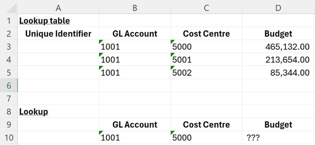
In Excel, most lookup functions are designed to accept only a single lookup criterion. However, in accounting, scenarios frequently arise where multiple criteria are essential. For instance, when looking up the budgeted amount for a specific expense category within a particular cost centre, both the general ledger account code and the cost centre serve as necessary lookup criteria. In this article, we will explore effective methods to perform multi-criteria lookups in Excel.
What is the workaround approach?
Take a look at the syntax of accountants' favourite function, VLOOKUP (see Microsoft's VLOOKUP documentation):
=VLOOKUP(lookup_criteria, lookup_table, column_index, [approximate_or_exact])In this function, only one argument is available for the lookup criteria. The same limitation applies to other popular functions like MATCH, LOOKUP, HLOOKUP, and even XLOOKUP.
To perform a multi-criteria lookup, a common approach is to combine multiple criteria into a single identifier, essentially creating a unique value that represents all necessary criteria. For example, instead of searching by first name and last name separately, you could combine them into a single full name and perform a lookup based on the full name.
Similarly, in an accounting context, if you need to look up data based on both account code and cost centre, you could create a unique identifier by joining these two (or more) fields together and using it as your lookup criterion. Here is how you can create a unique identifier by concatenating the values in columns B and C with a hyphen as a delimiter:
=B3&"-"&C3A worked example makes this clearer. Suppose your budget table lists an amount for each combination of account code and cost centre:
| Account code | Cost centre | Combined key | Budget |
|---|---|---|---|
| 6000 | CC-01 | 6000-CC-01 | S$1,500 |
| 6000 | CC-02 | 6000-CC-02 | S$2,300 |
| 6100 | CC-01 | 6100-CC-01 | S$4,750 |
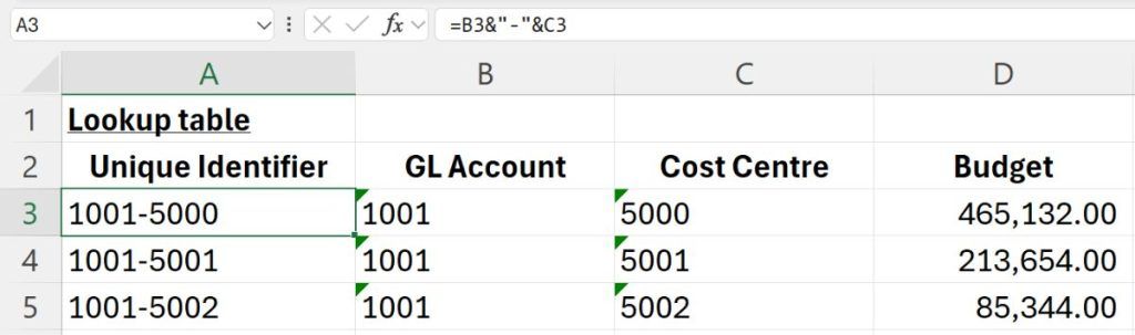
In the lookup function, we will do the same thing by concatenating the lookup criteria using a hyphen as a delimiter.

Creating a helper column (column A) may not be efficient in some situations, as it adds an extra step to apply formulas to new entries in the lookup table. If you are using the latest version of Excel, which includes XLOOKUP, you can perform the concatenation of columns directly within the XLOOKUP function. This is because of XLOOKUP's ability to handle dynamic arrays, allowing for more flexible and powerful lookups. To learn more about dynamic arrays, refer to my previous article, Dynamic Array Formulas In Excel. For a broader comparison of the two functions, see XLOOKUP or VLOOKUP?.
=XLOOKUP(B10&"-"&C10, B3:B5&"-"&C3:C5, D3:D5)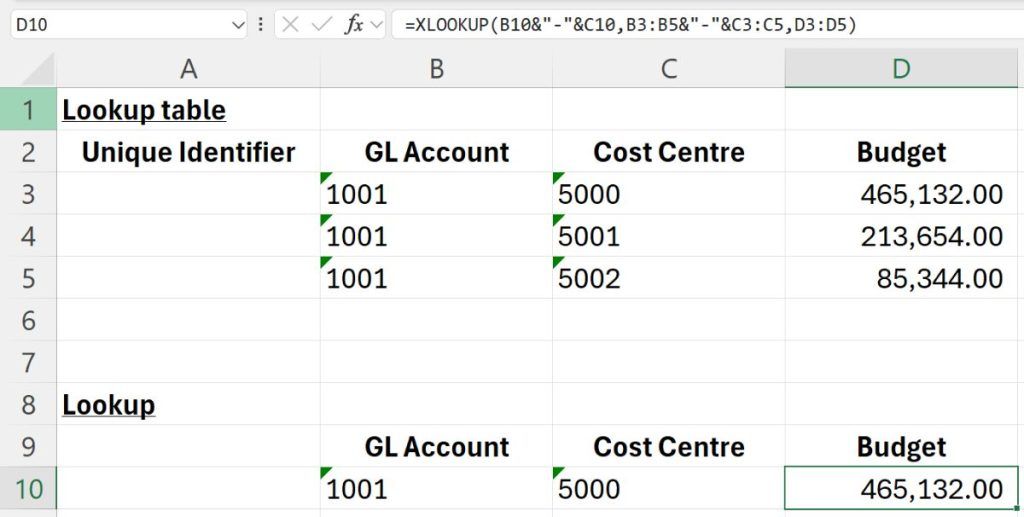
How do you choose a delimiter?
This workaround approach relies on creating a unique identifier by combining multiple criteria into a single value. However, selecting an appropriate delimiter is crucial to ensure accuracy. The delimiter you choose — whether it is a hyphen, underscore or another character — should be distinctive enough to prevent any overlap with the actual data in each column. For example, if one of your criteria contains hyphens as part of its normal data format, using a hyphen as a delimiter could lead to confusing or incorrect matches.
Which functions accept multiple criteria by design?
Another approach to a multi-criteria lookup is using functions that support multiple criteria by design. Two examples that we will explore here are SUMIFS and FILTER. These functions are more reliable and more efficient in a multi-criteria context. But each of them has some other limitations.
SUMIFS
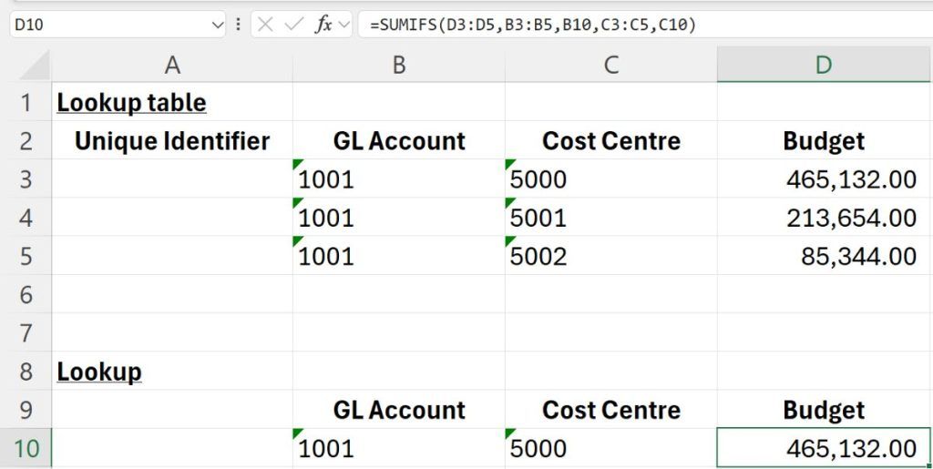
SUMIFS is another popular function used by accountants (see Microsoft's SUMIFS documentation). It sums up the values for entries in the lookup table that meet the criterion or criteria. The syntax is as follows:
=SUMIFS(value_range, criteria_range1, criteria1, [criteria_range2, criteria2], ...)The main limitation of SUMIFS is that it only returns numerical values. Additionally, if multiple occurrences of the criteria exist in the lookup table, SUMIFS will add all matching values together, which may not be suitable in cases where you need a single, distinct match rather than a cumulative total.
FILTER
The FILTER function in the latest version of Excel is more flexible, allowing you to perform a range of operations beyond simple lookups (see Microsoft's FILTER documentation). With FILTER, you can not only apply multiple criteria but also more complex conditions to filter and retrieve specific data sets dynamically. However, this added capability also introduces complexity.
Unlike more familiar functions that follow a straightforward syntax, FILTER requires a different approach for combining criteria. For example, using multiplication (*) for AND conditions and addition (+) for OR conditions within a formula can be confusing initially, especially for users accustomed to simpler functions. Additionally, as you add more layers of criteria, the formula can become more complex to manage and troubleshoot. While FILTER can handle sophisticated operations, its syntax may feel overwhelming for those new to dynamic arrays or advanced filtering techniques.
The FILTER syntax for multi-criteria scenarios is as follows:
=FILTER(value_range, (criteria_range1 = criteria1) * (criteria_range2 = criteria2), [if_empty])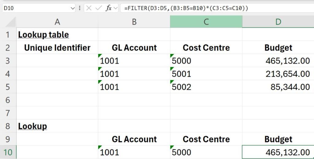
One key behaviour of the FILTER function to be aware of is its ability to return multiple matching entries. When multiple results meet the specified criteria, FILTER will return all of them, automatically spilling into adjacent rows or columns as needed. This dynamic array feature is powerful for generating lists of matches. However, if you are expecting only one result, the spilling behaviour may require extra management to prevent overlapping with other data on your sheet.
So which method should you use?
So, which one is better? There is no clear winner. However, in an accounting context, SUMIFS would likely be the most appropriate function when we work with numerical data.
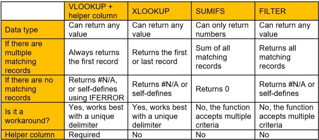
The possible solutions can be summarised as follows:
| Method | How it handles multiple criteria | Main limitation |
|---|---|---|
| VLOOKUP or XLOOKUP with a combined key | Concatenate the criteria into one unique identifier | Needs a helper column, or a modern Excel version for in-formula concatenation |
| SUMIFS | Accepts several criteria ranges by design | Returns numbers only; sums all matching rows |
| FILTER | Accepts several criteria and complex conditions | Harder syntax; spills multiple matches |
Frequently asked questions
This information has been prepared for general informational purposes only and is not intended to be relied upon as accounting, tax, or other professional advice.
Related articles
articles
Advanced Lookup: Wildcards
How accountants use Excel wildcards — the asterisk and question mark — to match account names and codes by pattern in SUMIF, VLOOKUP and XLOOKUP formulas.
articles
Dynamic Array Formulas in Excel: Unleashing the Power
How Excel dynamic array formulas such as FILTER and XLOOKUP spill results across cells, so accountants can build scalable, error-resistant templates and audit working papers.
articles
Two-Dimensional Lookup
A step-by-step guide to two-dimensional lookups in Excel: combine VLOOKUP with MATCH to retrieve a value by row and column, keep the formula dynamic, and tidy it with nesting.