Dynamic Array Formulas in Excel: Unleashing the Power
How Excel dynamic array formulas such as FILTER and XLOOKUP spill results across cells, so accountants can build scalable, error-resistant templates and audit working papers.

Xian Hui
23 June 2025
Quick answer
How do dynamic array formulas in Excel help accountants build scalable templates?
Dynamic array formulas, available in Microsoft 365, let a single formula spill its results across multiple cells instead of one. Functions such as FILTER, SORT and UNIQUE automatically expand and contract as your data changes. For accountants, this means scalable templates and working papers that adapt to varying numbers of rows without copying formulas down or filtering data by hand each period.
Dynamic Array Formulas in Excel: Unleashing the Power
Written by Ng Xian Hui, Founder of Backbone. Originally published on ISCA's Chartered Accountants Lab.
We accountants love templates because reusable templates save time. Train Excel to do a task once, and it will repeat the task for you afterwards. One key aspect when building templates is scalability. A good template adapts to varying amounts of data, minimising manual intervention when the numbers change.
For the longest time, formulas only returned a result in the very cell where you entered them; they did not automatically fill into other cells. If you wanted a formula on every line of a table, you had to copy it to each row by hand. When new data arrived, you updated the formulas again, which was inefficient and error-prone. If a report table had a variable number of rows, you had to write formulas for the maximum number of lines you might ever need, which limited scalability further.
Excel introduced dynamic array formulas in Microsoft 365. Beyond fixing those inefficiencies, let us explore their benefits and how to apply them to accounting use cases.
Key takeaways
- Dynamic array formulas automatically spill results into multiple cells, allowing more efficient data handling and scalable templates that adapt to varying data sizes without manual adjustment.
- Dynamic arrays take some learning for users used to traditional formulas, but the investment pays off in fewer manual updates, fewer errors and more reliable financial reports — helping to future-proof your accounting processes.
What are dynamic array formulas?
Dynamic array formulas in Excel can return multiple values at once. Unlike a traditional formula that outputs a single value in one cell, a dynamic array formula spills its results into multiple cells. This makes data manipulation far more versatile — a must-know if you are building templates for scalability.
There are three key aspects to dynamic array formulas.
New dynamic array functions
Excel introduced several new functions designed to work with dynamic arrays, including FILTER, SORT, UNIQUE and SEQUENCE. These functions generate arrays of values based on various criteria, and they automatically spill into the range of cells they need.
The spill range operator (#)
Excel introduced the spill range operator, the hash sign, to work with dynamic arrays. This operator lets you reference the entire spilled range of a dynamic array formula, rather than a single cell within it.
Range input
Many Excel functions now accept a range of cells as input rather than a single cell. This enhances their flexibility and power. For example, you can apply a lookup to an entire range of lookup values in a single formula, making calculations more efficient and less error-prone.
How do dynamic arrays help with audit working papers?
Let us demonstrate with a practical example: creating a lead schedule for audit working papers. Traditional Excel formulas would require you to copy a formula to each row of the schedule, and updating the data meant adjusting the formulas again by hand. That process was slow and prone to inconsistency.
The comparison below sums up the difference between the two approaches.
| Aspect | Traditional VLOOKUP method | Dynamic array FILTER method |
|---|---|---|
| Returning multiple matches | Not possible directly; needs an auto-filter and copy-paste | FILTER returns all matches and spills them automatically |
| Adding new rows | Copy the formula to every new row | The formula expands on its own |
| Retrieving related values | Copy the lookup down each row | A lookup with the # operator adjusts automatically |
| Reusing the template | Re-filter and re-copy for each section | Copy the sheet and change one input cell |
What did the traditional VLOOKUP method require?
Consider a lead schedule for audit working papers where you need a list of account numbers mapped to a particular lead schedule — K101 for property, plant and equipment, for example — then look up those account numbers in the chart of accounts for their descriptions.
VLOOKUP only returns one result, however many matches exist in the lookup table, and we usually have more than one account mapped to a single lead schedule. That makes it impossible for traditional lookup functions to return all relevant account numbers without awkward workarounds. So the most practical solution was to auto-filter the lookup table, then copy and paste the relevant account numbers into the lead schedule template.
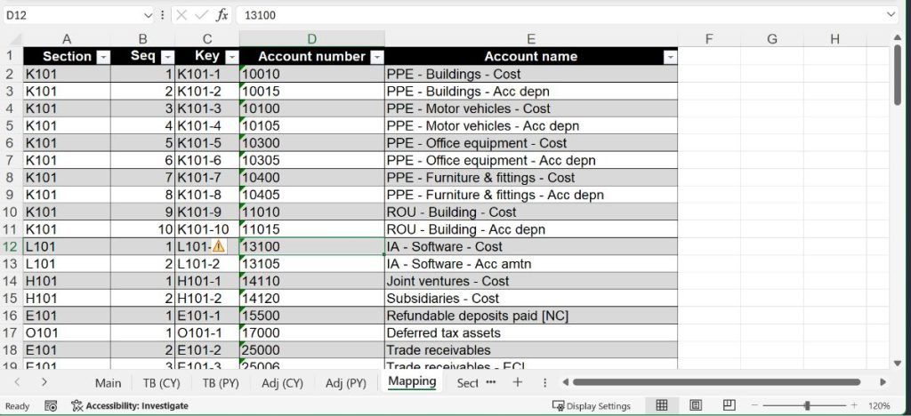
You could then use a VLOOKUP function to retrieve the account names from the chart of accounts. With more than 10 accounts, as in this example, you had to copy the formula in cell C7 down to every row.
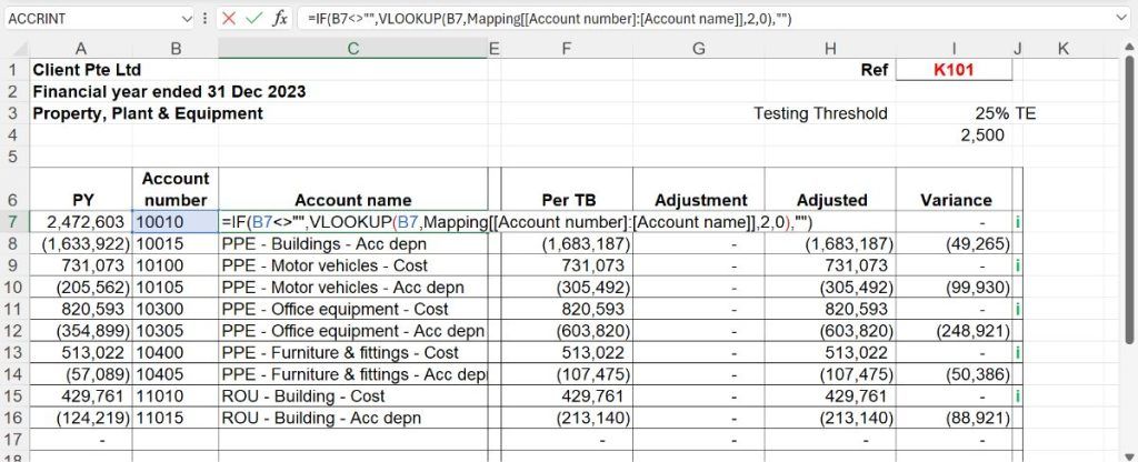
If you are wondering how to reference data by calling the column header, see Microsoft's documentation on structured references.
How does the FILTER method work?
Now let us use the dynamic array function FILTER for the same task.
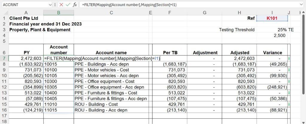
In cell B7, enter the FILTER function:
=FILTER(Mapping[Account number], Mapping[Section]=I1)When more than one result is found, this formula spills the results into multiple cells, showing every account number associated with the section specified in cell I1 of the lead schedule.
To retrieve the account names in column C, you can use XLOOKUP (or VLOOKUP) in cell C7. To make the lookup a dynamic array formula, add a # sign after the B7 reference instead of pointing at a single cell. This references the entire spill range starting from cell B7:
=XLOOKUP(B7#, Mapping[Account number], Mapping[Account name])If you give a range input to an argument that originally accepted only a single cell reference — such as the lookup value of XLOOKUP — the formula spills automatically. So if the FILTER function in cell B7 returns more account numbers, or fewer, the lookup adjusts accordingly.
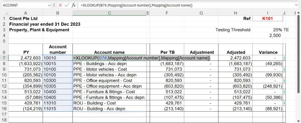
With this setup, the lookup dynamically adjusts to the number of account numbers returned by FILTER in B7, ensuring every relevant account name appears in column C. Here is how to populate columns F, G and H:
Cell F7: =SUMIFS(TB_CY[Net], TB_CY[Account number], B7#)
Cell G7: =SUMIFS(Adj_CY[Net], Adj_CY[Account number], B7#)
Cell H7: =F7#+G7#
Now you only need to copy the sheet and change I1 to another section to populate the data for the next section. There are no awkward workarounds and no manual filtering of relevant account numbers.
Which other dynamic array functions are useful?
Here are a few more dynamic array functions worth exploring at your own pace:
- UNIQUE — returns a list of unique values from a range or array.
- SORT — sorts the contents of a range or array.
- SEQUENCE — generates a list of sequential numbers in an array.
You can read more about these in Microsoft's guide to dynamic arrays and spilled array behaviour.
What should you watch out for with dynamic arrays?
Function arguments that accept ranges
This one is not intuitive. In column H, you would typically write =SUM(F7:G7). Adding a # operator after F7 and G7 — =SUM(F7#:G7#) — might look as though it should spill down through H16. It will not.
The SUM function accepts ranges as arguments. So when you add # operators to the references, SUM interprets it as a request to sum the entire ranges where the spill ends, making it equivalent to =SUM(F7:F16, G7:G16). A formula only auto-spills when its argument originally accepted a single cell reference. That is why we use =F7#+G7# rather than SUM.
Dynamic array references
You cannot use the spill range operator (#) to reference cells that are not part of a dynamic array result. Only dynamic array formulas produce spill ranges that the # operator can reference.
Spill blocking
If data already sits in cells where a dynamic array would normally spill, you get a #SPILL! error. Keep the spill range clear to avoid it.
Performance considerations
Dynamic arrays save user time and maintenance effort because they adjust automatically to changes in data size. Functions such as UNIQUE, FILTER and SEQUENCE handle tasks more efficiently than traditional workarounds. That said, on extremely large datasets or complex operations — for example, FILTER or SORTBY on very large tables — dynamic arrays can cause performance issues.
Conclusion
It has been a long wait for Excel fans, but dynamic array formulas are finally here, not only matching but in many ways exceeding similar features that have long existed in Google Sheets. These tools let accountants handle data more efficiently and accurately.
Dynamic arrays make it possible to build scalable templates that adapt effortlessly to varying data sizes and complexities. They do take some learning for users accustomed to traditional Excel formulas, but the time invested pays off through fewer manual updates, fewer errors and more reliable financial reports. Embrace dynamic arrays to streamline your accounting processes and keep your work efficient and future-proof.
Frequently asked questions
This information has been prepared for general informational purposes only and is not intended to be relied upon as accounting, tax, or other professional advice.
Related articles
articles
Automating the Final Mile of Report Generation
A beginner-friendly guide to using VBA in Excel to automate the final mile of report generation — decoupling a finished report from its working file so it is accurate, well formatted and ready to share.
articles
How do we see data analytics?
Data analytics only works when it starts with a clear purpose. Here is how we see it — define the problem first, plan your data steps together, and use only the tools you genuinely understand.
articles
Sending Reports Via Email With VBA
A practical guide to automating report emails from Excel with VBA, using a named table and Outlook to send messages and attachments to a list of recipients in one click.